Sentence embedding models

This page introduces the sentence embedding models under study and the evaluation architecture. The results of the study are presented on a separate page.

Introduction to sentence embedding

A crucial component in most natural language processing (NLP) applications is finding an expressive representation for text. Modern methods are typically based on sentence embeddings that map a sentence onto a numerical vector. The vector attempts to capture the semantic content of the text. If two sentences express a similar idea using different words, their representations (embedding vectors) should still be similar to each other.

Several methods for constructing these embeddings have been proposed in the literature. Interestingly, learned embeddings tend generalize quite well to other material and NLP tasks besides the ones they were trained on. This is fortunate, because it allows us to use pre-trained models and avoid expensive training. (A single training run on a modern, large-scale NLP model can cost up to tens of thousands of dollars).

Sentence embeddings are being applied on almost all NLP application areas. In information retrieval they are used for comparing the meanings of text snippets, machine translation uses sentence embeddings as an “intermediate language” when translating between two human languages and many classification and tagging applications are based on embeddings. With better representations it is possible to build applications that react more naturally to the sentiment and topic of written text.

Evaluated sentence embedding models

This study compares sentence embedding models which have a pre-trained Finnish variant publicly available. State-of-the-art models without a published Finnish variant, such as GPT-2 and XLNet, are not included in the evaluation.

The most important sentence embedding models can be divided into three categories: baseline bag-of-word models, models that are based on aggregating embeddings for the individual words in a sentence, and models that build a representation for a full sentence.

Bag-of-words (BoW)

TF-IDF. I’m using TF-IDF (term frequency-inverse document frequency) vectors as a baseline. A TF-IDF vector is a sparse vector with one dimension per each unique word in the vocabulary. The value for an element in a vector is an occurrence count of the corresponding word in the sentence multiplied by a factor that is inversely proportional to the overall frequency of that word in the whole corpus. The latter factor is meant to diminish the effect of very common words (mutta, ja, siksi, …) which are unlikely to tell much about the actual content of the sentence. The vectors are L2-normalized to reduce the effect of differing sentence lengths.

As a preprocessing, words are converted to their dictionary form (lemmatized). Unigrams and bigrams occurring less than k times are filtered out. The cutoff parameter k is optimized on the training data. Depending on the corpus this results in dimensionality (i.e. the vocabulary size) around 5000. TF-IDF vectors are very sparse, because one document usually contains only a small subset of all words in the vocabulary.

BoW models treat each word as an equivalent entity. They don’t consider the semantic meaning of words. For example, a BoW model doesn’t understand that a horse and a pony are more similar than a horse and a monocle. Next, we’ll move on to word embedding models that have been introduced to take the semantic information better into account.

Pooled word embeddings

A word embedding is a vector representation of a word. Words, which often occur in similar context (a horse and a pony), are assigned vector that are close by each other and words, which rarely occur in a similar context (a horse and a monocle), dissimilar vectors. The embedding vectors are dense, relatively low dimensional (typically 50-300 dimensions) vectors.

The embedding vectors are typically trained on a language modeling task: predict the presentation for a word given the representation of a few previous (and possibly following) words. This is a self-supervised task as the supervision signal is the order of the word in a document. The training requires just a large corpus of text documents. It is well established that word embeddings learned on a language modeling task generalize well to other downstream tasks: classification, part-of-speech tagging and so on.

Pooled word2vec. One of the earliest and still widely used word embedding model is the word2vec model (Mikolov, Chen, Corrado, & Dean, 2013). I’m using the Finnish word2vec vectors trained on the Finnish Internet Parsebank data by the Turku NLP research group. The embeddings are 300 dimensional.

There are several ways to get from the word embeddings to sentence embeddings. Perhaps, the most straight-forward idea is to aggregate the embeddings of each word that appears in a sentence, for example, by taking an element-wise average, minimum or maximum. These strategies are called average-pooling, min-pooling and max-pooling, respectively. Still another alternative is the concatenation of min- and max-pooled vectors. In this work, I’m evaluating average-pooled word2vec. Average-pooling performed better than the alternatives on a brief preliminary study on the TDT dataset. As this might be dataset-dependent, it’s a good idea to experiment with different pooling strategies.

Pooled FastText (Bojanowski, Grave, Joulin, & Mikolov, 2017) extends the word2vec by generating embeddings for subword units (character n-grams). By utilizing the subword structure, FastText aims to provide better embeddings for rare and out-of-vocabulary words. It should help particularly on morpheme-rich languages like Finnish (Finnish uses lots of inflections). The authors of FastText have published a Finnish model trained on Finnish subsets of Common Crawl and Wikipedia. I’m average-pooling the word embeddings to get an embedding for the sentence.

Researchers have proposed also other aggregation methods besides simple pooling. I’m evaluating two such proposals here: SIF and BOREP.

SIF. (Arora, Liang, & Ma, 2017) introduces a model called smooth inverse frequency (SIF). They propose taking a weighted average (weighted by a term related to the inverse document frequency) of the word embeddings in a sentence and then removing the projection of the first singular vector. This is derived from an assumption that the sentence has been generated by a random walk of a discourse vector on a latent word embedding space, and by including smoothing terms for frequent words.

BOREP. The idea of BOREP or bag of random embedding projections (Wieting & Kiela, 2019) is to project word embeddings to a random high-dimensional space and pool the projections there. The intuition is that casting things into a higher dimensional space tends to make them more likely to be linearly separable thus making the text classification easier. In the evaluations, I’m projecting to a 4096 dimensional space following the lead of the paper authors.

While word embeddings capture some aspects of semantics, pooling embeddings is quite a crude way of aggregating the meaning of a sentence. Pooling for example completely ignores the order of the words. The current state-of-the-art in NLP is deep learning models that take a whole sentence as an input and are thus capable of processing the full context of the sentence. Let’s take a look at two such models.

Contextual full sentence embeddings

FinBERT (Virtanen et al., 2019) is the influential BERT model (Bidirectional Encoder Representations from Transformers) (Devlin, Chang, Lee, & Toutanova, 2018) trained from scratch on Finnish texts. The BERT model consists of encoder transformer layers which are able to take the bi-directional context of each word into account. The model employs self-attention to focus on relevant context.

In the evaluations, the sentence embedding is the output vector from one of the last layers or the average of the last four layers. The optimal embedding layer is chosen separately for each task together with other hyperparameters. BERT also generates output embeddings for each input word, but these are not used in the evaluations, just the output layer of the special classification token. In the paraphrase and consecutive sentence evaluation tasks, which compare two sentences directly, both sentences are fed as input separated by a separator token to match how BERT was trained.

I’m using the Huggingface implementation of the pre-trained FinBERT (cased) model. The embedding dimensionality is 768.

LASER. As the second contextual sentence embedding method, I’ll evaluate LASER (Language-Agnostic SEntence Representations) by (Artetxe & Schwenk, 2018). It is specifically meant to learn language-agnostic sentence embeddings. It has a similar deep bi-directional architecture as BERT, but uses LSTM encoders instead of transformer blocks like BERT. I’m using the pre-trained model published by the LASER authors. It produces 1024 dimensional embedding vectors.

Sentence classifier architecture

The sentence embedding models are evaluated on sentence classification tasks (given a sentence output the class it belongs to) or sentence pair comparison tasks (given a pair of sentences output a binary yes/no judgment: are the two sentences paraphrases or do they belong to the same document). Sentence embedding models are combined with a task-specific classifier neural network.

The architecture used in the evaluations is show on the image below. The sentence embedding model under evaluation (the blue block) converts the sentence text into a sentence embedding vector which is the input for a task-specific classifier (the orange blocks). The classifier consists of a dense hidden layer with a sigmoid activation and a softmax output layer. Both layers are regularized by dropout. The dimensionality, weights and dropout probabilities of the classifier are optimized on the development dataset (separately for each task and embedding model) but the pre-trained sentence embedding model is keep fixed during the whole experiment.

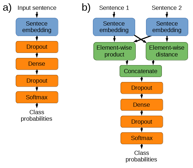
For sentence pair tasks (labeled as b) in the image), I’m using a technique introduced by (Tai, Socher, & Manning, 2015): first, sentence embeddings are generated for the two sentences separately, and then they are merged into a single feature vector that represents the pair (the green blocks). The merging is done as follows: Let the embeddings for the two sentences be called u and v. The feature vector for the pair is then generated as a concatenation of the element-wise product u ⊙ v and the element-wise absolute distance |u − v|. The concatenated feature vector is then used as the input for the classification part, like above. The FinBERT model is an exception. It has an integrated way of handling sentence pair tasks (see above).

The final evaluation results are computed on a test set that has not been used during the training.

The pre-trained sentence embedding models are treated as black box feature extractors that output embedding vectors. An alternative approach is to fine-tune a pre-trained embedding model by optimizing the full pipeline (usually with just a small learning rate for the embedding part). Feature extraction is computationally cheaper, but fine-tuning potentially adapts the embeddings better to various tasks. The relative performance of feature extraction and fine-tuning approaches depends on the similarity of the pre-training and target tasks (Peters, Ruder, & Smith, 2019) and its effects should be studied on each task separately. The current evaluation focuses only on the feature extraction strategy to understand what can be achieved on relatively low computational resources.

References

Arora, S., Liang, Y., & Ma, T. (2017). A simple but tough-to-beat baseline for sentence embeddings. In International conference on learning representations (ICLR 2017). Retrieved from https://openreview.net/forum?id=SyK00v5xx
Artetxe, M., & Schwenk, H. (2018). Massively multilingual sentence embeddings for zero-shot cross-lingual transfer and beyond. arXiv Preprint arXiv:1812.10464. Retrieved from https://arxiv.org/abs/1812.10464
Bojanowski, P., Grave, E., Joulin, A., & Mikolov, T. (2017). Enriching word vectors with subword information. Transactions of the Association for Computational Linguistics, 5, 135–146. Retrieved from https://arxiv.org/abs/1607.04606
Devlin, J., Chang, M.-W., Lee, K., & Toutanova, K. (2018). BERT: Pre-training of deep bidirectional transformers for language understanding. arXiv Preprint arXiv:1810.04805. Retrieved from https://arxiv.org/abs/1810.04805
Mikolov, T., Chen, K., Corrado, G. S., & Dean, J. (2013). Efficient estimation of word representations in vector space. In International conference on learning representations (ICLR 2013). Retrieved from https://arxiv.org/abs/1301.3781
Peters, M. E., Ruder, S., & Smith, N. A. (2019). To tune or not to tune? Adapting pretrained representations to diverse tasks. arXiv Preprint arXiv:1903.05987. Retrieved from https://arxiv.org/abs/1903.05987
Tai, K. S., Socher, R., & Manning, C. D. (2015). Improved semantic representations from tree-structured long short-term memory networks. In Association for computational linguistics (ACL 2015). Retrieved from https://nlp.stanford.edu/pubs/tai-socher-manning-acl2015.pdf
Virtanen, A., Kanerva, J., Ilo, R., Luoma, J., Luotolahti, J., Salakoski, T., … Pyysalo, S. (2019). Multilingual is not enough: BERT for finnish. arXiv Preprint arXiv:1912.07076. Retrieved from https://arxiv.org/abs/1912.07076
Wieting, J., & Kiela, D. (2019). No training required: Exploring random encoders for sentence classification. arXiv Preprint arXiv:1901.10444. Retrieved from https://arxiv.org/abs/1901.10444